


Over the past decade, the 19th century science-of-counting has been resurrected to provide a combinatorial derivation of conventional Machine Learning that uniquely generalizes statistics to probability theory, allows energy to enter or exit the system, and processes any time-series to return a complete set of scientific (thermodynamic) measurements as deductive reality. And now with a plausible way to explain and generalize Machine Learning for time-series, we observe that “Machine” and “Artificial Intelligence” are too prominent in this case, because in the science-of-counting computers only do what they have done from the beginning: evaluate built-in functions. The derivation of the functions is human intelligence, not artificial intelligence. In the science-of-counting “scientific machine learning” will be simplified to scientific learning.
Conventional machine learning is effective in static, closed world applications, but cannot accommodate changing environments, where energy can enter or exit, or, where energy is stored for later release. Energy allowed to enter or exit a system should also allow emotional energy to enter and exit, as it is the principle and obvious source of human energy that can both affect dynamics and anticipate a need. Scientific learning is the combinatorial science-of-counting evaluated on time-series that permit both energy flow and energy storage, and reduces correctly to statistics when there is no energy entering or exiting the system.
The human mind (intuition, intellect and emotions) is a gift capable to understand deductive Reality. On the other hand, human invention plays no role at all, because everything follows from deduction, freed from human bias and caprice.
By examining problems that share the same overall mathematical structure as Scientific Learning, the power grid is historically based on the science-of-counting with a key engineering assumption/simplification that the average of the strain vanishes, so that we can ignore the strain. And strain can be ignored only at statistical equilibrium, when the system is just as likely to go up as to go down. The traditional power grid could ignore strain, because power generation was controlled and predictable. But given renewable energy sources, the next generation of power grid must recognize and manage power grid strains, along with supply and demand.
When applied to a “need”, say, electrical power, Scientific Learning becomes the Science of Giving and Receiving. With both supply and demand time-series given, the power grid realizes the Science of Giving and Receiving, and inherits the analytical benefits. The science of giving and receiving is used to re-architect the electrical power grid for non-equilibrium operation that can better support variable energy sources (renewables). The power grid of the future is a re-engineering problem that is not solved by government policy alone.
Supply and Demand Interactions
The functions that define the relationship between energy, momentum and velocity, E=pv, are deduced in the science-of-counting (the dispersion relation). To manage supply and demand the same analysis is deductively extended to interactions as well. A high-level picture of the interaction science is presented here.
Given a time-series for electrical energy supply (in MWh), \(n_A\), there are natural coordinates (an eigenbasis) in scientific learning that define the Expected Supply and its associated Expected Strain. Similarly, given a time-series for energy demand (in MWh), \(n_B\), the Expected Demand and its associated Expect Strain are defined. The Lagrangian below enforces supply and demand measurements as constraints, \(\cal{L}_A\) and \(\cal{L}_B\), and moreover adds the constraints for interaction measurements, with the Lagrange multipliers \(\lambda_{AB}\) and the \(\sigma_{AB}\) terms below.
\[\begin{align} \cal{L} &= \cal{L}_A + \cal{L}_B - \lambda_{AB}\,<n_A\,n_B> - \,\sigma_{AB}\,<v_A\,v_B>. \end{align}\]If the supply and demand time-series are independent, that is, there is no interaction between the two, then the time-series would report that the couplings \(\lambda_{AB}\) and \(\sigma_{AB}\) are both equal to zero, and that \(p(n_A n_B) = p(n_A)p(n_B)\). In truth, of course, supply and demand are highly coupled and interact non-trivially. For better insight, we introduce the interaction function, \(\Lambda\), of two time-series defined by
\[\begin{align} \Lambda \equiv \frac{p(n_A)p(n_B)}{p(n_A n_B)}, \end{align}\]so that when \(\Lambda = 1\), the equation reduces correctly to the definition of probability independence. In general, scientific learning derives the interaction function algebraically, as a plane cubic curve that determines how the various momenta (normalized to also be probabilities) must fit together and change in concert (as a Tschirnhausen cubic):
\[\begin{align} p^2(n_A n_B)= \Bigg[1-\frac{p(n_A)p(n_B)}{p(n_A n_B)} \Bigg]\;p(n_A)p(n_B) &\quad \Rightarrow\quad p(n_A n_B) = \Lambda (1-\Lambda) \\ &\quad \Rightarrow\quad \Lambda = \frac{1}{2} \pm \sqrt{\frac{1}{4} - p(n_A n_B)}. \end{align}\]See the interaction diagram and coupling curve below.
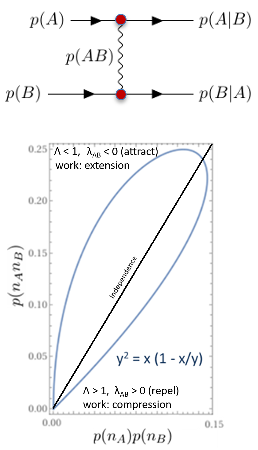
Using the following identities,
\[\begin{align} \frac{y}{x} = \frac{p(n_A n_B)}{p(n_A)p(n_B)} = \frac{p(n_A\vert n_B)}{p(n_A)} = \frac{p(n_B\vert n_A)}{p(n_B)}, \end{align}\]the curve is the same but the axis labels \(x\) and \(y\) define a different problem: forward and backward scattering, supply needed for demand, demand needed for supply, respectively. An analysis with live time-series data is being prepared for publication.
To Give and To Receive
The introduction of money breaks the deductive structure of scientific learning, which we have worked hard to preserve. The moment we introduce currency, models are introduced, in this case, exchange rate models that convert money to displacement energy. Expect every business process to have its own exchange rate: spend for a displacement energy. Exchange rate models imply some degree of control through spend, from which we will manage supply and demand scientifically.
Giving should meet both physical and spiritual needs, including instruction, counsel, comfort and forgiveness. For St. Thomas Aquinas, giving and receiving are not merely economic or social acts. They are moral, spiritual and relational realities that mirror the very life of God.